

The Wild World of Modeling
All code for this presentation can be found at this repo here!
Some model example web applications can be found here and also here.
1 Overview
This is a presentation that I gave (April 28, 2016) to a graduate student led temporal and spatial modeling seminar at UC Berkeley. Here I present a number of ideas in mathematical and statistical modeling from the point of view of both theoretical and practical implementation.
Quick reference on model thinking
1.1 Concepts
I plan to cover topics in implementing model thinking both conceptually and numerically, including:
- discrete vs continuous time
- parametric vs non parametric models
- feature importance and model validity: p-values vs residuals, k-near neighbors clustering for variable importance, cross-validation etc
- Anscombe’s quartet
I plan to describe some issues in the practical implementation of modeling, including:
- value of interpretation: e.g. decision trees vs random forest
- accessibility: ease of use vs statistical / mathematical stability - desktop software vs web based approaches
1.2 A Disease Example
We will use a reoccurring example throughout this presentation of a disease model. This model was implemented and taught by myself and others from the Getz lab - Wayne Getz at UC Berkeley - at TeenTechSF 2016.
Let’s assume you have 1000 individuals within some population - for example within a typical American High School during Flu season. Of the 1000 students, 999 are healthy, flu-less, studious individuals. However, there is 1 infected individual! In our model of this disease we conceptualize this as 999 susceptible and 1 infected.
2 The Issues of Time
There are two general ways to conceptualize the use of time within a model:
discrete time - the model consistently increments in t + 1 with each iteration of the simulation
continuous time - the model uses dt to integrate over “slopes” of time in a continuous manner
2.1 Discrete Time
We can think about discrete time in a simple step-wise manner. The simulation has a set of values, e.g. the number of susceptible students and the number of infected students, at time t. Well what happens when we move to the next day (assuming our model clock is in units days)? We can step from time t to time t + 1 and update all simulation variables / parameters before or after the time iteration. This is an important distinction! If we are updating beforehand than any functions that take time are using time = t and NOT time = t + 1 like they would with post-updating! This can cause major differences in simulation output and behavior.
2.2 Continuous Time
We can think about continuous time as a differential equation problem. This can seem daunting…but have no fear because the visual language of the Nova software is here to help! More below…
Instead of updating the model clock by steps, we integrate over a slope from time = t to time = t + 1 through n number of dt “steps” / “bins”. What this means is that the integration of your model parameters occurs as a function of your dt (change of time) “step”. These dt values can be thought of more as bins. It is the same way you would integrate on paper in a calculus class (or whatever class you may be integrating things in).
2.3 Change Over Time
Deciding which time approach a simulation takes is so underrated and so very, very important!
Discrete time disease model - web app
Continuous time disease model - web app
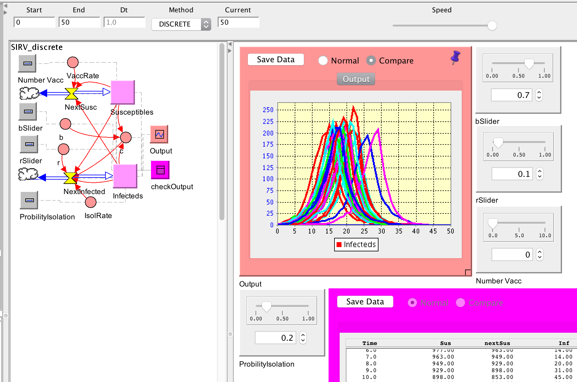
2.4 Our Disease Model in Nova
Here our disease model using discrete time - 50 runs:
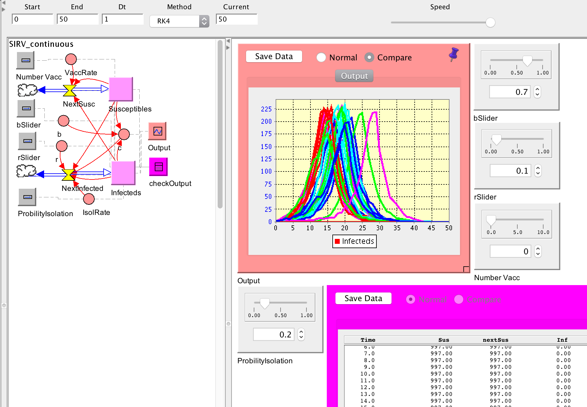
And here is the same model using continuous time with dt = 1 - 50 runs:
And finally - same continuous model but with dt = 0.1 - 50 runs:
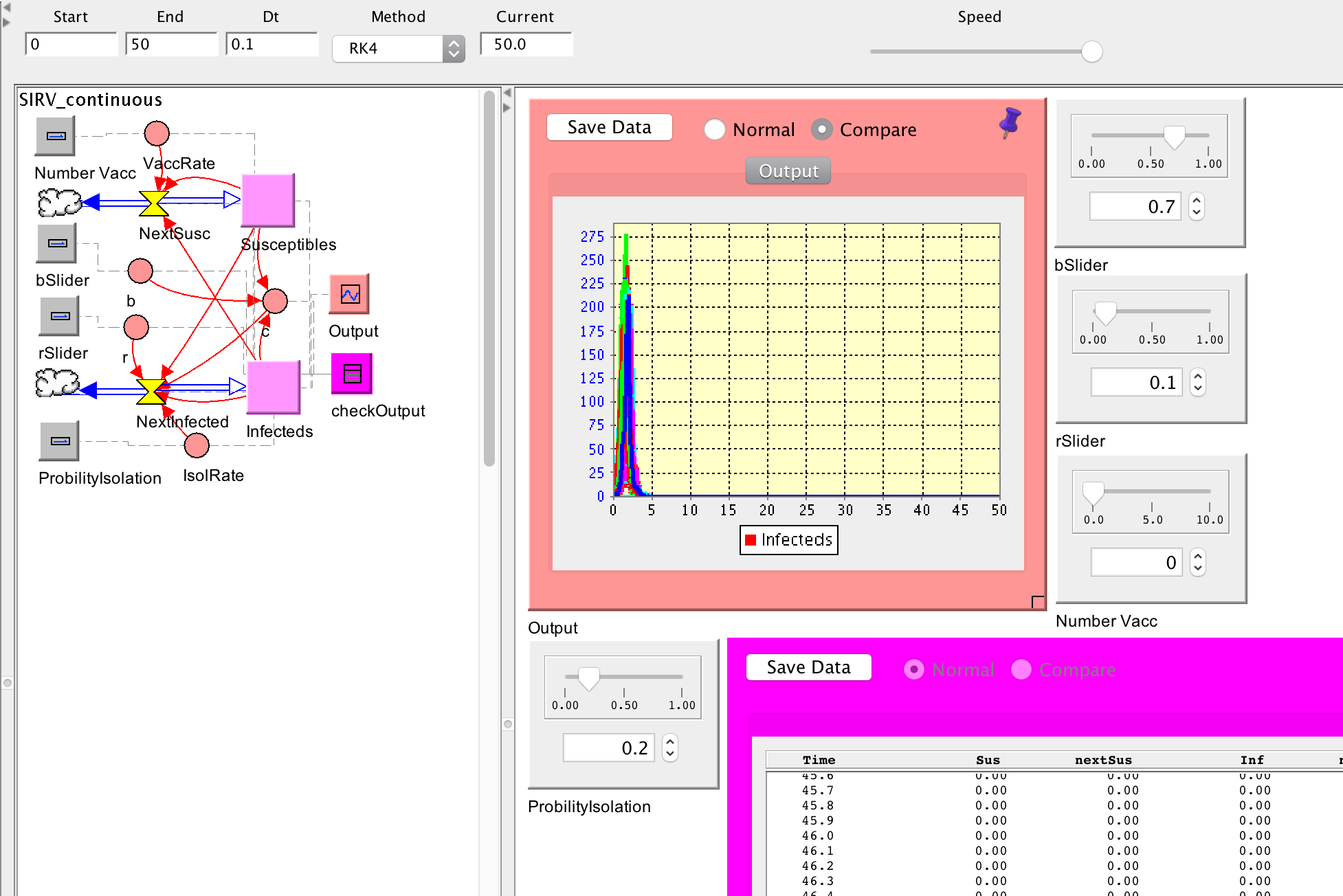
We could also see web-application versions of the discrete and continuous with dt = 0.1 models (see below for links).
3 Parametric or Non-parametric
3.1 Linear Assumptions
Linear regression is a non-parametric statistical model. Linear models assume the data is linear…but much more! Linear models assume the following:
- there is a linear relationship between the response (Y) and the predictors (X)
- the errors / noise of the predictors / variables / x are equal
- these errors (above) are independent and they are Gaussian (i.e. variance distribution)
3.2 Reference into Anscombe’s Quartet
One of my favorite statistical examples / illustrative exercises:
Notes about linear model assumptions and Anscombe’s quartet
4 Model Validity
Let’s take linear models as an example - extending from what is described above.
4.1 Wrong Time for Linear Regression
Here we can check out both the binomial and tree-methods files - examples / referenced from a wonderful set of R tutorials.
But one of the most famous and obvious examples can be seen in Anscombe’s quartet below.
4.2 Anscombe’s Quartet
Are p-values and other forms of model validity testing really valid?
A bit more detailed of a review of Anscombe’s quartet
A very detailed / heavily mathematical review of Anscombe’s quartet